Image Classification with PyTorch and Cleanlab#
This quickstart tutorial demonstrates how to find issues in image classification data. Here we use the Fashion-MNIST dataset (60,000 images of fashion products from 10 categories), but you can replace this with your own image classification dataset and still follow the same tutorial.
Overview of what we’ll do in this tutorial:
Build a simple PyTorch neural net.
Use cross-validation to compute out-of-sample predicted probabilities (
pred_probs) and feature embeddings (features) for each image in the dataset.Utilize these
pred_probsandfeaturesto identify potential issues within the dataset using theDatalabclass from cleanlab. The issues found by cleanlab include mislabeled examples, near duplicates, outliers, and image-specific problems such as excessively dark or low information images.
Quickstart
Already have a ML model? Run cross-validation to get out-of-sample pred_probs and provide features (embeddings of the data). Then use the code below to find any potential issues in your dataset (you can also run this code with one of pred_probs or features instead of both, but less issue types will be considered).
from cleanlab import Datalab

lab = Datalab(data=your_dataset, label_name="column_name_of_labels")  # include `image_key` to detect low-quality images
lab.find_issues(pred_probs=pred_probs, features=features)

lab.report()
1. Install and import required dependencies#
You can use pip to install all packages required for this tutorial as follows:
!pip install matplotlib torch torchvision datasets
!pip install "cleanlab[image]"
# We install cleanlab with extra dependencies for image data
# Make sure to install the version corresponding to this tutorial
# E.g. if viewing master branch documentation:
#     !pip install "cleanlab[image] @ git+https://github.com/cleanlab/cleanlab.git"
[2]:
from torch.utils.data import DataLoader, TensorDataset, Subset
import torch
import torch.nn as nn
import torch.optim as optim

from sklearn.model_selection import StratifiedKFold
import numpy as np
import matplotlib.pyplot as plt

from tqdm.autonotebook import tqdm
import math
import time
import multiprocessing

from cleanlab import Datalab
from datasets import load_dataset
2. Fetch and normalize the Fashion-MNIST dataset#
Load train split of the fashion_mnist dataset and view the number of rows and columns in the dataset
[3]:
dataset = load_dataset("fashion_mnist", split="train")
dataset
Downloading data: 100%|██████████| 30.9M/30.9M [00:00<00:00, 102MB/s]
Downloading data: 100%|██████████| 5.18M/5.18M [00:00<00:00, 48.2MB/s]
[3]:
Dataset({
    features: ['image', 'label'],
    num_rows: 60000
})
Get number of classes in the dataset
[4]:
num_classes = len(dataset.features["label"].names)
num_classes
[4]:
10
[5]:
# Convert PIL image to torch tensors
transformed_dataset = dataset.with_format("torch")


# Apply transformations
def normalize(example):
    example["image"] = (example["image"] / 255.0).unsqueeze(0)
    return example


transformed_dataset = transformed_dataset.map(normalize, num_proc=multiprocessing.cpu_count())
Convert the transformed dataset to a torch dataset. Torch datasets are more efficient with dataloading in practice.
[6]:
torch_dataset = TensorDataset(transformed_dataset["image"], transformed_dataset["label"])
Bringing Your Own Data (BYOD)?
Load any huggingface dataset or your local image folder dataset, apply relevant transformations, and continue with the rest of the tutorial.
3. Define a classification model#
Here, we define a simple neural network with PyTorch. Note this is just a toy model to ensure quick runtimes for the tutorial, you can replace it with any other (larger) PyTorch network.
[7]:
class Net(nn.Module):
    def __init__(self):
        super().__init__()
        self.cnn = nn.Sequential(
            nn.Conv2d(1, 6, 5),
            nn.ReLU(),
            nn.BatchNorm2d(6),
            nn.MaxPool2d(2, 2),
            nn.Conv2d(6, 16, 5, bias=False),
            nn.ReLU(),
            nn.BatchNorm2d(16),
            nn.MaxPool2d(2, 2),
        )
        self.linear = nn.Sequential(nn.LazyLinear(128), nn.ReLU())
        self.output = nn.Sequential(nn.Linear(128, num_classes))

    def forward(self, x):
        x = self.embeddings(x)
        x = self.output(x)
        return x

    def embeddings(self, x):
        x = self.cnn(x)
        x = torch.flatten(x, 1)  # flatten all dimensions except batch
        x = self.linear(x)
        return x
Helper methods for cross validation (click to expand)
# Note: This pulldown content is for docs.cleanlab.ai, if running on local Jupyter or Colab, please ignore it.

# Set device
device = torch.device("cuda" if torch.cuda.is_available() else "cpu")


# Method to calculate validation accuracy in each epoch
def get_test_accuracy(net, testloader):
    net.eval()
    accuracy = 0.0
    total = 0.0

    with torch.no_grad():
        for data in testloader:
            images, labels = data["image"].to(device), data["label"].to(device)

            # run the model on the test set to predict labels
            outputs = net(images)

            # the label with the highest energy will be our prediction
            _, predicted = torch.max(outputs.data, 1)
            total += labels.size(0)
            accuracy += (predicted == labels).sum().item()

    # compute the accuracy over all test images
    accuracy = 100 * accuracy / total
    return accuracy


# Method for training the model
def train(trainloader, testloader, n_epochs, patience):
    model = Net()

    criterion = nn.CrossEntropyLoss()
    optimizer = optim.AdamW(model.parameters())

    model = model.to(device)

    best_test_accuracy = 0.0

    for epoch in range(n_epochs):  # loop over the dataset multiple times
        start_epoch = time.time()
        running_loss = 0.0

        for _, data in enumerate(trainloader):
            # get the inputs; data is a dict of {"image": images, "label": labels}

            inputs, labels = data["image"].to(device), data["label"].to(device)

            # zero the parameter gradients
            optimizer.zero_grad()

            # forward + backward + optimize
            outputs = model(inputs)
            loss = criterion(outputs, labels)
            loss.backward()
            optimizer.step()

            running_loss += loss.detach().cpu().item()

        # Get accuracy on the test set
        accuracy = get_test_accuracy(model, testloader)

        if accuracy > best_test_accuracy:
            best_epoch = epoch

        # Condition for early stopping
        if epoch - best_epoch > patience:
            print(f"Early stopping at epoch {epoch + 1}")
            break

        end_epoch = time.time()

        print(
            f"epoch: {epoch + 1} loss: {running_loss / len(trainloader):.3f} test acc: {accuracy:.3f} time_taken: {end_epoch - start_epoch:.3f}"
        )
    return model


# Method for computing out-of-sample embeddings
def compute_embeddings(model, testloader):
    embeddings_list = []

    with torch.no_grad():
        for data in tqdm(testloader):
            images, labels = data["image"].to(device), data["label"].to(device)

            embeddings = model.embeddings(images)
            embeddings_list.append(embeddings.cpu())

    return torch.vstack(embeddings_list)


# Method for computing out-of-sample predicted probabilities
def compute_pred_probs(model, testloader):
    pred_probs_list = []

    with torch.no_grad():
        for data in tqdm(testloader):
            images, labels = data["image"].to(device), data["label"].to(device)

            outputs = model(images)
            pred_probs_list.append(outputs.cpu())

    return torch.vstack(pred_probs_list)
4. Prepare the dataset for K-fold cross-validation#
To find label issues based on pred_probs, we recommend out-of-sample predictions, which can be produced via K-fold cross-validation. To ensure this tutorial runs quickly, we set K and other important neural network training hyperparameters to small values here. Use larger values to get good results in practice!
[10]:
K = 3  # Number of cross-validation folds. Set to small value here to ensure quick runtimes, we recommend 5 or 10 in practice for more accurate estimates.
n_epochs = 2  # Number of epochs to train model for. Set to a small value here for quick runtime, you should use a larger value in practice.
patience = 2  # Parameter for early stopping. If the validation accuracy does not improve for this many epochs, training will stop.
train_batch_size = 64  # Batch size for training
test_batch_size = 512  # Batch size for testing
num_workers = multiprocessing.cpu_count()  # Number of workers for data loaders

# Create k splits of the dataset
kfold = StratifiedKFold(n_splits=K, shuffle=True, random_state=0)
splits = kfold.split(transformed_dataset, transformed_dataset["label"])

train_id_list, test_id_list = [], []

for fold, (train_ids, test_ids) in enumerate(splits):
    train_id_list.append(train_ids)
    test_id_list.append(test_ids)
5. Compute out-of-sample predicted probabilities and feature embeddings#
We use cross-validation to compute out-of-sample predicted probabilities separately for each dataset fold. However, we use only one model to generate embeddings for all the images across the full dataset. This ensures all feature embeddings lie in the same representation space for more accurate detection of data issues. Here we embed all the data using our model trained in the first cross-validation fold, but you could also train a separate embedding model on the full dataset.
[11]:
pred_probs_list, embeddings_list = [], []
embeddings_model = None

for i in range(K):
    print(f"\nTraining on fold: {i+1} ...")

    # Create train and test sets and corresponding dataloaders
    trainset = Subset(torch_dataset, train_id_list[i])
    testset = Subset(torch_dataset, test_id_list[i])

    trainloader = DataLoader(
        trainset,
        batch_size=train_batch_size,
        shuffle=False,
        num_workers=num_workers,
        pin_memory=True,
    )
    testloader = DataLoader(
        testset, batch_size=test_batch_size, shuffle=False, num_workers=num_workers, pin_memory=True
    )

    # Train model
    model = train(trainloader, testloader, n_epochs, patience)
    if embeddings_model is None:
        embeddings_model = model

    # Compute out-of-sample embeddings
    print("Computing feature embeddings ...")
    fold_embeddings = compute_embeddings(embeddings_model, testloader)
    embeddings_list.append(fold_embeddings)

    print("Computing predicted probabilities ...")
    # Compute out-of-sample predicted probabilities
    fold_pred_probs = compute_pred_probs(model, testloader)
    pred_probs_list.append(fold_pred_probs)

print("Finished Training")


# Combine embeddings and predicted probabilities from each fold
features = torch.vstack(embeddings_list).numpy()

logits = torch.vstack(pred_probs_list)
pred_probs = nn.Softmax(dim=1)(logits).numpy()
Training on fold: 1 ...
epoch: 1 loss: 0.482 test acc: 86.720 time_taken: 4.955
epoch: 2 loss: 0.329 test acc: 88.195 time_taken: 4.652
Computing feature embeddings ...
Computing predicted probabilities ...
Training on fold: 2 ...
epoch: 1 loss: 0.493 test acc: 87.060 time_taken: 4.676
epoch: 2 loss: 0.330 test acc: 88.505 time_taken: 4.699
Computing feature embeddings ...
Computing predicted probabilities ...
Training on fold: 3 ...
epoch: 1 loss: 0.476 test acc: 86.340 time_taken: 4.861
epoch: 2 loss: 0.328 test acc: 86.310 time_taken: 4.566
Computing feature embeddings ...
Computing predicted probabilities ...
Finished Training
Reorder rows of the dataset based on row order in features and pred_probs. Carefully ensure your ordering of the dataset matches these objects! Make sure that the columns of your pred_probs are properly ordered with respect to the ordering of classes, which for Datalab is: lexicographically sorted by class name.
[12]:
indices = np.hstack(test_id_list)
dataset = dataset.select(indices)
7. Use cleanlab to find issues#
Based on the out-of-sample predicted probabilities and feature embeddings from our ML model, cleanlab can automatically detect issues in our labeled dataset.
Here we use cleanlab’s Datalab class to find issues in our data. Datalab supports several data formats, in this tutorial we have a Hugging Face Dataset. Datalab takes in two optional dataset arguments: label_name, which corresponds to the column containing labels (if your dataset is labeled), and image_key, corresponding to the name of a key in your vision dataset to access the raw images. When you provide these optional arguments, Datalab will audit your dataset for more
types of issues than it would by default.
[13]:
lab = Datalab(data=dataset, label_name="label", image_key="image")
The find_issues method can automatically infer the types of issues to be checked for based on the provided arguments. Here, we provide features and pred_probs as arguments. If you want to check for a specific issue type, you can do so using the issue_types argument. Check the documentation for a more comprehensive guide on find_issues method.
[14]:
lab.find_issues(features=features, pred_probs=pred_probs)
Finding null issues ...
Finding label issues ...
Finding outlier issues ...
Fitting OOD estimator based on provided features ...
Finding near_duplicate issues ...
Finding non_iid issues ...
Finding class_imbalance issues ...
Finding underperforming_group issues ...
Finding dark, light, low_information, odd_aspect_ratio, odd_size, grayscale, blurry images ...
Removing grayscale from potential issues in the dataset as it exceeds max_prevalence=0.1

Audit complete. 7714 issues found in the dataset.
View report#
After the audit is complete, we can view a high-level report of detected data issues.
[15]:
lab.report()
Here is a summary of the different kinds of issues found in the data:

     issue_type  num_issues
        outlier        3772
          label        3585
 near_duplicate         175
low_information         166
           dark          16

Dataset Information: num_examples: 60000, num_classes: 10


---------------------- outlier issues ----------------------

About this issue:
        Examples that are very different from the rest of the dataset
    (i.e. potentially out-of-distribution or rare/anomalous instances).


Number of examples with this issue: 3772
Overall dataset quality in terms of this issue: 0.3651

Examples representing most severe instances of this issue:
       is_outlier_issue  outlier_score
27080              True   3.873833e-07
40378              True   6.915575e-07
25316              True   1.390277e-06
2090               True   3.751164e-06
14999              True   3.881301e-06


----------------------- label issues -----------------------

About this issue:
        Examples whose given label is estimated to be potentially incorrect
    (e.g. due to annotation error) are flagged as having label issues.


Number of examples with this issue: 3585
Overall dataset quality in terms of this issue: 0.9569

Examples representing most severe instances of this issue:
       is_label_issue  label_score given_label  predicted_label
11262            True     0.000003        Coat  T - shirt / top
19228            True     0.000010       Dress            Shirt
32657           False     0.000013         Bag            Dress
21282           False     0.000016         Bag            Dress
53564            True     0.000018    Pullover  T - shirt / top


------------------ near_duplicate issues -------------------

About this issue:
        A (near) duplicate issue refers to two or more examples in
    a dataset that are extremely similar to each other, relative
    to the rest of the dataset.  The examples flagged with this issue
    may be exactly duplicated, or lie atypically close together when
    represented as vectors (i.e. feature embeddings).


Number of examples with this issue: 175
Overall dataset quality in terms of this issue: 0.6321

Examples representing most severe instances of this issue:
       is_near_duplicate_issue  near_duplicate_score near_duplicate_sets  distance_to_nearest_neighbor
30968                     True              0.001267             [30659]                      0.000022
30659                     True              0.001267             [30968]                      0.000022
47824                     True              0.001454              [3370]                      0.000026
3370                      True              0.001454             [47824]                      0.000026
54565                     True              0.001854  [9762, 258, 47139]                      0.000033


Removing grayscale from potential issues in the dataset as it exceeds max_prevalence=0.5
------------------ low_information images ------------------

Number of examples with this issue: 166
Examples representing most severe instances of this issue:
----------------------- dark images ------------------------

Number of examples with this issue: 16
Examples representing most severe instances of this issue:
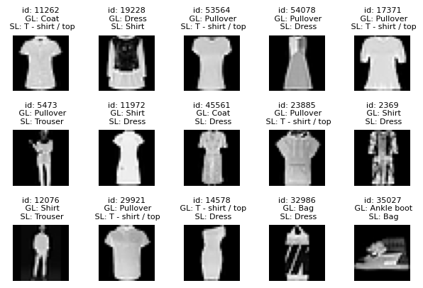
Label issues#
Let’s first inspect mislabeled examples in the dataset. Such errors occur when the given label for an image is incorrect, usually due to mistakes made by data annotators. Cleanlab automatically detects mislabeled data that you can correct to improve your dataset.
For each type of issue that Cleanlab detects, you can use the get_issues method to see which examples in the dataset exhibit this type of issue (and how severely). Let’s see which images in our dataset are estimated to be mislabeled:
[16]:
label_issues = lab.get_issues("label")
label_issues.head()
[16]:
| is_label_issue | label_score | given_label | predicted_label | |
|---|---|---|---|---|
| 0 | False | 0.166980 | T - shirt / top | Dress |
| 1 | False | 0.986195 | T - shirt / top | T - shirt / top |
| 2 | False | 0.997205 | Sandal | Sandal |
| 3 | False | 0.948781 | Sandal | Sandal |
| 4 | False | 0.999358 | Dress | Dress |
The above dataframe contains a label_score for each example in the dataset. These numeric quality scores lie between 0 and 1, where lower scores indicate examples more likely to be mislabeled. It contains a boolean column is_label_issue specifying whether or not each example appears to have a label issue (indicating it is likely mislabeled).
Filter the label_issues DataFrame to see which examples have label issues, and sort by label_score(in ascending order) to see the most likely mislabeled examples first.
[17]:
label_issues_df = label_issues.query("is_label_issue").sort_values("label_score")
label_issues_df.head()
[17]:
| is_label_issue | label_score | given_label | predicted_label | |
|---|---|---|---|---|
| 11262 | True | 0.000003 | Coat | T - shirt / top |
| 19228 | True | 0.000010 | Dress | Shirt |
| 53564 | True | 0.000018 | Pullover | T - shirt / top |
| 54078 | True | 0.000022 | Pullover | Dress |
| 17371 | True | 0.000025 | Pullover | T - shirt / top |
We define a helper method plot_label_issue_examples to visualize results. (click to expand)
# Note: This pulldown content is for docs.cleanlab.ai, if running on local Jupyter or Colab, please ignore it.

def plot_label_issue_examples(label_issues_df, num_examples=15):
    ncols = 5
    nrows = int(math.ceil(num_examples / ncols))

    _, axes = plt.subplots(nrows=nrows, ncols=ncols, figsize=(1.5 * ncols, 1.5 * nrows))
    axes_list = axes.flatten()
    label_issue_indices = label_issues_df.index.values

    for i, ax in enumerate(axes_list):
        if i >= num_examples:
            ax.axis("off")
            continue
        idx = int(label_issue_indices[i])
        row = label_issues.loc[idx]
        ax.set_title(
            f"id: {idx}\n GL: {row.given_label}\n SL: {row.predicted_label}",
            fontdict={"fontsize": 8},
        )
        ax.imshow(dataset[idx]["image"], cmap="gray")
        ax.axis("off")
    plt.subplots_adjust(hspace=0.7)
    plt.show()
View most likely examples with label errors#
Here we define GL : given label in the original dataset SL : suggested alternative label by cleanlab
[19]:
plot_label_issue_examples(label_issues_df, num_examples=15)
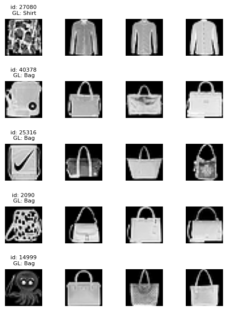
Outlier issues#
Datalab also detects atypical images lurking in our dataset. Such outliers are significantly different from the majority of the dataset and may have an outsized impact on how models fit to this data.
Similarly to the previous section, we filter the outlier_issues DataFrame to find examples that are considered to be outliers. We then sort the filtered results by their outlier quality score, where examples with the lowest scores are those that appear least typical relative to the rest of the dataset.
[20]:
outlier_issues_df = lab.get_issues("outlier")
outlier_issues_df = outlier_issues_df.query("is_outlier_issue").sort_values("outlier_score")
outlier_issues_df.head()
[20]:
| is_outlier_issue | outlier_score | |
|---|---|---|
| 27080 | True | 3.873833e-07 |
| 40378 | True | 6.915575e-07 |
| 25316 | True | 1.390277e-06 |
| 2090 | True | 3.751164e-06 |
| 14999 | True | 3.881301e-06 |
View most severe outliers#
In this visualization, the first image in every row shows the potential outlier, while the remaining images in the same row depict typical instances from the corresponding class.
We define a helper method plot_outlier_issues_examples to visualize results. (click to expand)
# Note: This pulldown content is for docs.cleanlab.ai, if running on local Jupyter or Colab, please ignore it.

def plot_outlier_issues_examples(outlier_issues_df, num_examples):
    ncols = 4
    nrows = num_examples
    N_comparison_images = ncols - 1

    def sample_from_class(label, number_of_samples, index):
        index = int(index)

        non_outlier_indices = (
            label_issues.join(outlier_issues_df)
            .query("given_label == @label and is_outlier_issue.isnull()")
            .index
        )
        non_outlier_indices_excluding_current = non_outlier_indices[non_outlier_indices != index]

        sampled_indices = np.random.choice(
            non_outlier_indices_excluding_current, number_of_samples, replace=False
        )

        label_scores_of_sampled = label_issues.loc[sampled_indices]["label_score"]

        top_score_indices = np.argsort(label_scores_of_sampled.values)[::-1][:N_comparison_images]

        top_label_indices = sampled_indices[top_score_indices]

        sampled_images = [dataset[int(i)]["image"] for i in top_label_indices]

        return sampled_images

    def get_image_given_label_and_samples(idx):
        image_from_dataset = dataset[idx]["image"]
        corresponding_label = label_issues.loc[idx]["given_label"]
        comparison_images = sample_from_class(corresponding_label, 30, idx)[:N_comparison_images]

        return image_from_dataset, corresponding_label, comparison_images

    count = 0
    images_to_plot = []
    labels = []
    idlist = []
    for idx, row in outlier_issues_df.iterrows():
        idx = row.name
        image, label, comparison_images = get_image_given_label_and_samples(idx)
        labels.append(label)
        idlist.append(idx)
        images_to_plot.append(image)
        images_to_plot.extend(comparison_images)
        count += 1
        if count >= nrows:
            break

    ncols = 1 + N_comparison_images
    fig, axes = plt.subplots(nrows=nrows, ncols=ncols, figsize=(1.5 * ncols, 1.5 * nrows))
    axes_list = axes.flatten()
    for i, ax in enumerate(axes_list):
        if i % ncols == 0:
            ax.set_title(f"id: {idlist[i // ncols]}\n GL: {labels[i // ncols]}", fontdict={"fontsize": 8})
        ax.imshow(images_to_plot[i], cmap="gray")
        ax.axis("off")
    plt.subplots_adjust(hspace=0.7)
    plt.show()
[22]:
plot_outlier_issues_examples(outlier_issues_df, num_examples=5)
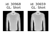
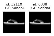
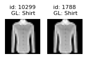
Near duplicate issues#
Datalab also detects which examples are (near) duplicates of other examples in the dataset. Near duplicate images in a dataset can lead to model overfitting and have an outsized impact on evaluation metrics (especially when you have duplicates between training and test splits).
The near_duplicate_issues DataFrame tells us which examples are considered to be nearly duplicated in the dataset (including exact duplicates as well). We can sort all images via the near_duplicate_score which quantifies how severe this issue is for each image (lower values indicate more severe instances of a type of issue, in this case, how similar the image is to its closest neighbor in the dataset).
This allows us to visualize examples in the dataset that are considered nearly duplicated, along with their highly similar counterparts.
[23]:
near_duplicate_issues_df = lab.get_issues("near_duplicate")
near_duplicate_issues_df = near_duplicate_issues_df.query("is_near_duplicate_issue").sort_values(
    "near_duplicate_score"
)
near_duplicate_issues_df.head()
[23]:
| is_near_duplicate_issue | near_duplicate_score | near_duplicate_sets | distance_to_nearest_neighbor | |
|---|---|---|---|---|
| 30659 | True | 0.001267 | [30968] | 0.000022 |
| 30968 | True | 0.001267 | [30659] | 0.000022 |
| 3370 | True | 0.001454 | [47824] | 0.000026 |
| 47824 | True | 0.001454 | [3370] | 0.000026 |
| 9762 | True | 0.001854 | [54565, 258, 47139] | 0.000033 |
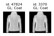
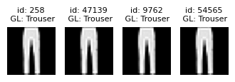
View sets of near duplicate images#
We define a helper method plot_near_duplicate_issue_examples to visualize results. (click to expand)
# Note: This pulldown content is for docs.cleanlab.ai, if running on local Jupyter or Colab, please ignore it.

def plot_near_duplicate_issue_examples(near_duplicate_issues_df, num_examples=3):
    nrows = num_examples
    seen_id_pairs = set()

    def get_image_and_given_label_and_predicted_label(idx):
        image = dataset[idx]["image"]
        label = label_issues.loc[idx]["given_label"]
        predicted_label = label_issues.loc[idx]["predicted_label"]
        return image, label, predicted_label

    count = 0
    for idx, row in near_duplicate_issues_df.iterrows():
        image, label, predicted_label = get_image_and_given_label_and_predicted_label(idx)
        duplicate_images = row.near_duplicate_sets
        nd_set = set([int(i) for i in duplicate_images])
        nd_set.add(int(idx))

        if nd_set & seen_id_pairs:
            continue

        _, axes = plt.subplots(1, len(nd_set), figsize=(len(nd_set), 3))
        for i, ax in zip(list(nd_set), axes):
            label = label_issues.loc[i]["given_label"]
            ax.set_title(f"id: {i}\n GL: {label}", fontdict={"fontsize": 8})
            ax.imshow(dataset[i]["image"], cmap="gray")
            ax.axis("off")
        seen_id_pairs.update(nd_set)
        count += 1
        if count >= nrows:
            break

    plt.show()
[25]:
plot_near_duplicate_issue_examples(near_duplicate_issues_df, num_examples=5)
Learn more about handling near duplicates detected in a dataset from the FAQ.
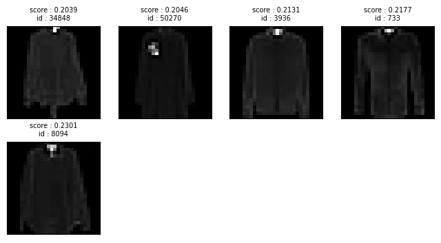
Dark images#
Datalab can also detect low-quality images in the dataset, such as those that are abnormally dark. It can be challenging for both annotators and models to assign a proper class label for low-quality data, which can hamper model training and testing.
The dark_issues DataFrame reveals which examples are considered to be abnormally dark. We can sort them via the dark_score which quantifies how severe this issue is for each image (lower values indicate more severe instances of a type of issue). This allows us to visualize images in the dataset considered to be too dark (you might consider omitting such low-quality examples from a training dataset).
[26]:
dark_issues = lab.get_issues("dark")
dark_issues_df = dark_issues.query("is_dark_issue").sort_values("dark_score")
dark_issues_df.head()
[26]:
| dark_score | is_dark_issue | |
|---|---|---|
| 34848 | 0.203922 | True |
| 50270 | 0.204588 | True |
| 3936 | 0.213098 | True |
| 733 | 0.217686 | True |
| 8094 | 0.230118 | True |
View top examples of dark images#
We define a helper method plot_image_issue_examples to visualize results. (click to expand)
# Note: This pulldown content is for docs.cleanlab.ai, if running on local Jupyter or Colab, please ignore it.

def plot_image_issue_examples(issues_df, num_examples=15):
    ncols = 5
    nrows = int(math.ceil(num_examples / ncols))

    _, axes = plt.subplots(nrows=nrows, ncols=ncols, figsize=(1.5 * ncols, 1.5 * nrows))
    axes_list = axes.flatten()
    issue_indices = issues_df.index.values

    for i, ax in enumerate(axes_list):
        if i >= num_examples:
            ax.axis("off")
            continue
        idx = int(issue_indices[i])
        label = label_issues.loc[idx]["given_label"]
        predicted_label = label_issues.loc[idx]["predicted_label"]
        ax.set_title(
            f"id: {idx}\n GL: {label}\n SL: {predicted_label}",
            fontdict={"fontsize": 8},
        )
        ax.imshow(dataset[idx]["image"], cmap="gray")
        ax.axis("off")

    plt.subplots_adjust(hspace=0.7)
    plt.show()
[28]:
plot_image_issue_examples(dark_issues_df, num_examples=5)
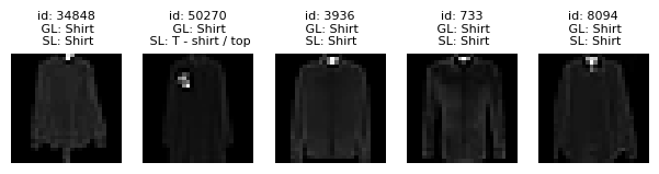
We can see from above examples that too dark images can also lead to label errors as it is difficult to see the contents of the image clearly.
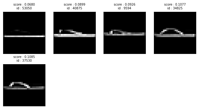
Low information images#
Other types of low-quality images that Datalab can automatically detect include images whose information content is low. Low information images can hamper model generalization if they are present disproportionately in some classes.
The lowinfo_issues DataFrame reveals which images are considered to be low information. We can sort them via the low_information_score which quantifies how severe this issue is for each image (lower values indicate more severe instances of a type of issue). This allows us to visualize the images in our dataset containing the least amount of information (you might consider omitting such low-quality examples from a training dataset).
[29]:
lowinfo_issues = lab.get_issues("low_information")
lowinfo_issues_df = lowinfo_issues.query("is_low_information_issue").sort_values(
    "low_information_score"
)
lowinfo_issues_df.head()
[29]:
| low_information_score | is_low_information_issue | |
|---|---|---|
| 53050 | 0.067975 | True |
| 40875 | 0.089929 | True |
| 9594 | 0.092601 | True |
| 34825 | 0.107744 | True |
| 37530 | 0.108516 | True |
[30]:
plot_image_issue_examples(lowinfo_issues_df, num_examples=5)
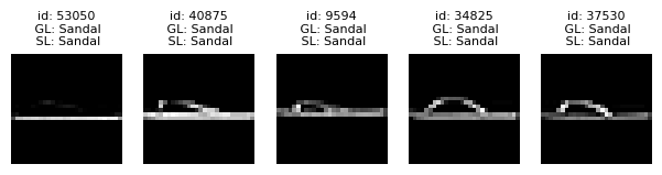
Here we can see a lot of low information images belong to the Sandal class.
Easy Mode#
Cleanlab is most effective when you run this code with a good ML model. Try to produce the best ML model you can for your data (instead of the toy model from this tutorial). If you don’t know the best ML model for your data, try Cleanlab Studio which will automatically produce one for you. Super easy to use, Cleanlab Studio is no-code platform for data-centric AI that automatically: detects data issues (more types of issues than this cleanlab package), helps you quickly correct these data issues, confidently labels large subsets of an unlabeled dataset, and provides other smart metadata about each of your data points – all powered by a system that automatically trains/deploys the best ML model for your data. Try it for free!