Finding Label Errors in Object Detection Datasets#
This 5-minute quickstart tutorial demonstrates how to find potential label errors in object detection datasets. In object detection data, each image is annotated with multiple bounding boxes. Each bounding box surrounds a physical object within an image scene, and is annotated with a given class label.
Using such labeled data, we train a model to predict the locations and classes of objects in an image. An example notebook to train the object detection model whose predictions we rely on in this tutorial is available here. These predictions can subsequently be input to cleanlab in order to identify mislabeled images and a quality score quantifying our confidence in the overall annotations for each image.
After correcting these label issues, you can train an even better version of your model without changing your training code!
This tutorial uses a subset of the COCO (Common Objects in Context) dataset which has images of everyday scenes and considers objects from the 5 most popular classes: car, chair, cup, person, traffic light.
Overview of what we we’ll do in this tutorial
Score images based on their overall label quality (i.e. our confidence each image is correctly labeled) using
cleanlab.object_detection.rank.get_label_quality_scoresEstimate which images have label issues using
cleanlab.object_detection.filter.find_label_issuesVisually review images + labels using
cleanlab.object_detection.summary.visualize
Quickstart
Already have labels and predictions in the proper format? Just run the code below to find label issues in your object detection dataset.
from cleanlab.object_detection.filter import find_label_issues
from cleanlab.object_detection.rank import get_label_quality_scores

# To get boolean vector of label issues for all images
has_label_issue = find_label_issues(labels, predictions)

# To get label quality scores for all images
label_quality_scores = get_label_quality_scores(labels, predictions)
1. Install required dependencies and download data#
You can use pip to install all packages required for this tutorial as follows
!pip install matplotlib
!pip install cleanlab
# Make sure to install the version corresponding to this tutorial
# E.g. if viewing master branch documentation:
#     !pip install git+https://github.com/cleanlab/cleanlab.git
[2]:
%%capture
from huggingface_hub import hf_hub_download
import zipfile
import os

# Download files from HuggingFace Hub
labels_path = hf_hub_download('Cleanlab/object-detection-tutorial', 'labels.pkl', repo_type="dataset")
predictions_path = hf_hub_download('Cleanlab/object-detection-tutorial', 'predictions.pkl', repo_type="dataset")
images_path = hf_hub_download('Cleanlab/object-detection-tutorial', 'example_images.zip', repo_type="dataset")

# Extract images to the correct location
# The zip file contains an example_images/ folder, so we extract it and then move contents
with zipfile.ZipFile(images_path, 'r') as zip_ref:
    zip_ref.extractall('temp_extract/')

# Move images from nested directory to target directory
import shutil
if os.path.exists('temp_extract/example_images/'):
    if os.path.exists('example_images/'):
        shutil.rmtree('example_images/')
    shutil.move('temp_extract/example_images/', 'example_images/')
    shutil.rmtree('temp_extract/')
else:
    # Fallback: extract directly if structure is different
    with zipfile.ZipFile(images_path, 'r') as zip_ref:
        zip_ref.extractall('example_images/')
[3]:
import pickle
from cleanlab.object_detection.filter import find_label_issues
from cleanlab.object_detection.rank import (
    _separate_label,
    _separate_prediction,
    get_label_quality_scores,
    issues_from_scores,
)
from cleanlab.object_detection.summary import visualize
2. Format data, labels, and model predictions#
We begin by loading labels and predictions for our dataset, which are the only inputs required to find label issues with cleanlab. Note that the predictions should be out-of-sample, which can be obtained for every image in a dataset via K-fold cross-validation.
In a separate example notebook (link), we trained a Detectron2 object detection model and used it to obtain predictions on a held-out validation dataset whose labels we audit here.
Note: If you want to find all the mislabeled images across the entire COCO dataset, you can first execute our other example notebook that uses K-fold cross-validation to produce out-of-sample predictions for every image, then use those labels and predictions below.
[4]:
IMAGE_PATH = './example_images/'  # path to raw image files downloaded above

# Load pickle files
with open(labels_path, 'rb') as f:
    labels = pickle.load(f)
with open(predictions_path, 'rb') as f:
    predictions = pickle.load(f)
In object detection datasets, each given label is a made up of bounding box coordinates and a class label. A model prediction is also made up of a bounding box and predicted class label, as well as the model confidence (probability estimate) in its prediction. To detect label issues, cleanlab requires given labels for each image, and the corresponding model predictions for the image (but not the image itself).
Here’s what an example looks like in our dataset. We visualize the given and predicted labels (in red and blue) for this image using the cleanlab.object_detection.summary.visualize method.
[5]:
import os

image_to_visualize = 8  # change this to view other images
image_path = IMAGE_PATH + labels[image_to_visualize]['seg_map']

# Check if the image file exists before trying to visualize
if os.path.exists(image_path):
    visualize(image_path, label=labels[image_to_visualize], prediction=predictions[image_to_visualize], overlay=False)
else:
    print(f"Image file not found: {image_path}")
    print("Skipping visualization - this is expected during documentation build.")

The required format of these labels and predictions matches what popular object detection frameworks like MMDetection and Detectron2 expect. Recall the 5 possible class labels in our dataset are: car, chair, cup, person, traffic light. These classes are represented as (zero-indexed) integers 0,1,…,4.
labels is a list where for the i-th image in our dataset, labels[i] is a dictionary containing: key labels – a list of class labels for each bounding box in this image and key bboxes – a numpy array of the bounding boxes’ coordinates. Each bounding box in labels[i]['bboxes'] is in the format [x1,y1,x2,y2] format with respect to the image matrix where (x1,y1) corresponds to the top-left corner of the box and (x2,y2) the bottom-right (E.g. XYXY in
Keras, Detectron 2).
Let’s see what labels[i] looks like for our previous example image:
[6]:
labels[image_to_visualize]
[6]:
{'bboxes': array([[201.96, 101.71, 334.78, 334.68]], dtype=float32),
 'labels': array([3]),
 'bboxes_ignore': array([], shape=(0, 4), dtype=float32),
 'masks': [[[290.44,
    200.04,
    286.59,
    213.5,
    285.63,
    224.08,
    290.44,
    231.77,
    293.32,
    235.62,
    289.48,
    251.97,
    282.74,
    266.39,
    281.78,
    271.2,
    280.82,
    277.93,
    279.86,
    287.55,
    277.93,
    299.09,
    276.97,
    307.75,
    276.97,
    321.21,
    281.78,
    326.02,
    290.44,
    330.83,
    286.59,
    333.71,
    263.51,
    334.68,
    261.59,
    319.29,
    257.74,
    295.25,
    251.97,
    290.44,
    251.97,
    283.7,
    250.05,
    283.7,
    243.31,
    303.9,
    243.31,
    316.4,
    243.31,
    319.29,
    247.16,
    323.14,
    251.01,
    326.02,
    249.08,
    328.91,
    227.93,
    327.94,
    226.0,
    323.14,
    226.96,
    313.52,
    226.96,
    303.9,
    226.0,
    293.32,
    216.39,
    283.7,
    226.0,
    236.58,
    228.89,
    226.96,
    232.73,
    219.27,
    239.47,
    216.39,
    240.43,
    209.65,
    242.35,
    202.92,
    240.43,
    185.61,
    230.81,
    198.11,
    219.27,
    215.42,
    218.31,
    224.08,
    220.23,
    229.85,
    217.35,
    237.54,
    213.5,
    238.5,
    207.73,
    239.47,
    204.84,
    239.47,
    201.96,
    237.54,
    201.96,
    228.89,
    205.81,
    224.08,
    206.77,
    220.23,
    218.31,
    191.38,
    219.27,
    185.61,
    223.12,
    180.8,
    226.0,
    175.03,
    229.85,
    167.34,
    231.77,
    159.64,
    236.86,
    153.25,
    240.46,
    151.71,
    253.35,
    149.13,
    254.9,
    147.07,
    250.26,
    143.46,
    247.16,
    140.88,
    244.59,
    124.39,
    244.59,
    115.11,
    246.65,
    109.44,
    249.74,
    104.81,
    256.44,
    102.23,
    262.11,
    101.71,
    268.29,
    101.71,
    273.96,
    101.71,
    277.06,
    101.71,
    283.76,
    108.41,
    284.79,
    110.48,
    287.88,
    119.24,
    286.85,
    122.33,
    286.85,
    126.97,
    286.85,
    132.64,
    286.85,
    136.76,
    285.82,
    145.52,
    284.27,
    150.16,
    286.33,
    151.71,
    290.97,
    155.83,
    293.03,
    173.35,
    297.67,
    180.05,
    317.25,
    190.87,
    319.32,
    191.9,
    326.53,
    192.42,
    329.62,
    192.93,
    332.2,
    196.03,
    334.26,
    201.18,
    334.78,
    207.88,
    329.11,
    209.94,
    326.53,
    205.82,
    324.47,
    203.24,
    323.44,
    202.21,
    320.86,
    202.21,
    316.22,
    203.76,
    314.68,
    203.24,
    313.65,
    200.67,
    307.46,
    199.63,
    297.67,
    198.6,
    294.58,
    197.06,
    291.49,
    197.06,
    290.97,
    196.03]]],
 'seg_map': '000000481413.jpg'}
predictions is a list where the predictions output by our model for the i-th image: predictions[i] is a list/array of shape (K,). Here K is the number of classes in the dataset (same for every image) and predictions[i][k] is of shape (M,5), where M is the number of bounding boxes predicted to contain objects of class k (in image i, differs between images). The five columns of predictions[i][k] correspond to [x1,y1,x2,y2,pred_prob] format with respect to
the image matrix for each bounding box predicted by the model. Here (x1,y1) corresponds to the top-left corner of the box and (x2,y2) the bottom-right (E.g. XYXY in Keras, Detectron 2). The last column, pred_prob is the model confidence in its predicted label of class k for this box. Since our dataset has
K = 5 classes, we have: predictions[i].shape = (5,).
Let’s see what predictions[i] looks like for our previous example image:
[7]:
predictions[image_to_visualize]
[7]:
array([array([], shape=(0, 5), dtype=float32),
       array([], shape=(0, 5), dtype=float32),
       array([], shape=(0, 5), dtype=float32),
       array([[204.42398  , 103.44503  , 337.29968  , 336.21005  ,   0.9978472]],
             dtype=float32)                                                      ,
       array([], shape=(0, 5), dtype=float32)], dtype=object)
Once you have labels and predictions in the appropriate formats, you can find label issues with cleanlab for any object detection dataset!
3. Use cleanlab to find label issues#
Given labels and predictions from our trained model, cleanlab can automatically find mislabeled images in the dataset. In object detection, we consider an image mislabeled if any of its bounding boxes or their class labels are incorrect (including if the image contains any overlooked objects which should’ve been annotated with a box)
Images may be mislabeled because annotators:
overlooked an object (forgot to annotate a bounding box around a depicted object)
chose the wrong class label for an annotated box in the correct location
imperfectly drew the bounding box such that its location is incorrect
Cleanlab is expected to flag images that exhibit any of these annotation errors as having label issues. More severe annotation errors are expected to produce lower cleanlab label quality scores closer to 0. Let’s first estimate which images have label issues:
[8]:
label_issue_idx = find_label_issues(labels, predictions, return_indices_ranked_by_score=True)

num_examples_to_show = 5 # view this many images flagged with the most severe label issues
label_issue_idx[:num_examples_to_show]
Pruning 0 predictions out of 138 using threshold==0.0. These predictions are no longer considered as potential candidates for identifying label issues as their similarity with the given labels is no longer considered.
[8]:
array([50, 16, 31, 29, 45])
The above code identifies which images have label issues, returning a list of their indices. This is because we specified the return_indices_ranked_by_score argument which sorts these indices by the estimated label quality of each image. Below we describe how to directly estimate the label quality scores of each image.
Note: You can omit the return_indices_ranked_by_score argument for find_label_issues() to instead return a Boolean mask for the entire dataset (True entries in this mask correspond to images with label issues)
Get label quality scores#
Cleanlab can also compute scores for each image to estimate our confidence that it has been correctly labeled. These label quality scores range between 0 and 1, with smaller values indicating examples whose annotation is more likely to be wrong in some way.
Each image in the dataset receives a label quality score. These scores are useful for prioritizing which images to review; if you have too little time, first review the images with the lowest label quality scores.
[9]:
scores = get_label_quality_scores(labels, predictions)
scores[:num_examples_to_show]
Pruning 0 predictions out of 138 using threshold==0.0. These predictions are no longer considered as potential candidates for identifying label issues as their similarity with the given labels is no longer considered.
[9]:
array([0.97489622, 0.70610878, 0.98764951, 0.88899237, 0.99085805])
We can also use the label quality scores to flag which images have label issues based on a threshold. Here we convert these per-image scores into an array of indices corresponding to images flagged with label issues, sorted by label quality score, in the same format returned by find_label_issues()
[10]:
issue_idx = issues_from_scores(scores, threshold=0.5)  # lower threshold will return fewer (but more confident) label issues
issue_idx[:num_examples_to_show], scores[issue_idx][:num_examples_to_show]
[10]:
(array([50, 16, 31, 29, 45]),
 array([6.95569726e-05, 9.03354841e-05, 8.57510169e-04, 1.58447666e-03,
        2.39755858e-01]))
4. Use ObjectLab to visualize label issues#
Finally, we can visualize images with potential label errors via cleanlab’s visualize() function. To enhance the visualization, you can supply a class_names dictionary to include as a legend and turn off overlay to see the given and predicted labels side by side.
[11]:
issue_to_visualize = issue_idx[0]  # change this to view other images
class_names = {"0": "car", "1": "chair", "2": "cup", "3":"person", "4": "traffic light"}

label = labels[issue_to_visualize]
prediction = predictions[issue_to_visualize]
score = scores[issue_to_visualize]
image_path = IMAGE_PATH + label['seg_map']

print(image_path, '| idx', issue_to_visualize , '| label quality score:', score, '| is issue: True')
if os.path.exists(image_path):
    visualize(image_path, label=label, prediction=prediction, class_names=class_names, overlay=False)
else:
    print(f"Image file not found: {image_path}")
    print("Skipping visualization - this is expected during documentation build.")
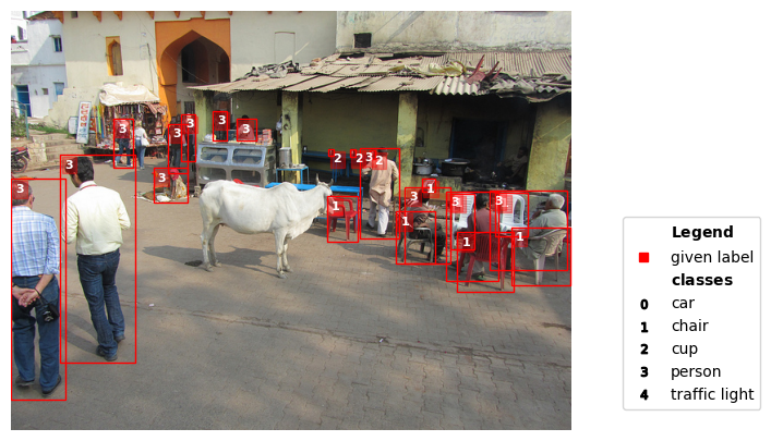
./example_images/000000009483.jpg | idx 50 | label quality score: 6.95569726168054e-05 | is issue: True
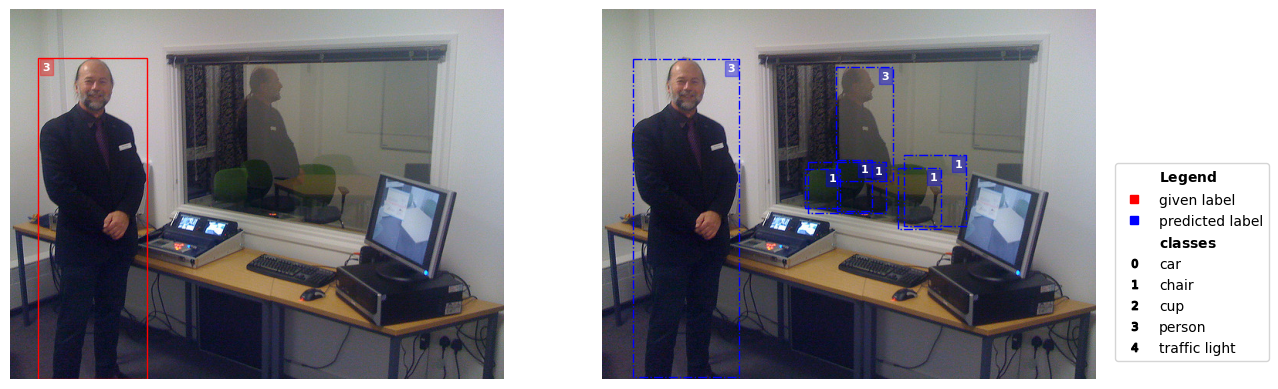
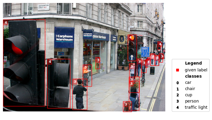
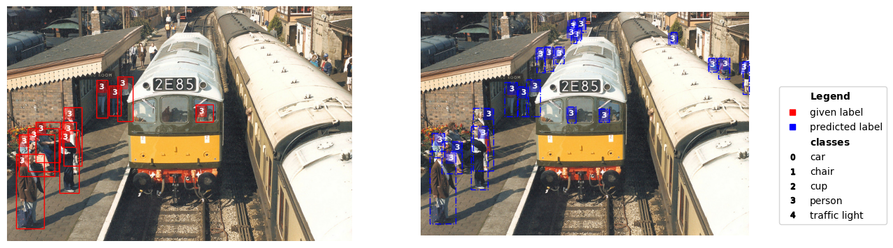
The visualization depicts the given label (original image annotation which cleanlab identified as problematic) in red on the left and the model-predicted label in blue on the right. Each bounding box contains a class-index number in the top corner indicating which object class that bounding box was annotated/predicted to contain.
This image has a low label quality score and is marked as an error. On closer inspection we notice the annotator missed the reflection of the person in the mirror that the model identified. Additionally, the chairs visible in the reflection were not annotated.
Notice examples where the predictions and labels are more similar have higher quality scores than those that are missmatched, and are less likeley to be marked as issues and the number of boxes is agnostic to the score.
Better trained models will lead to better label error detection but you don’t need a near perfect model to identify label issues.
Different kinds of label issues identified by ObjectLab#
Now lets view the first few images in our vaidation dataset that are clearly marked as issues and see what various inconsistencies between the given and predicted label we can spot.
[12]:
issue_to_visualize = issue_idx[1]
label = labels[issue_to_visualize]
prediction = predictions[issue_to_visualize]
score = scores[issue_to_visualize]

image_path = IMAGE_PATH + label['seg_map']
print(image_path, '| idx', issue_to_visualize , '| label quality score:', score, '| is issue: True')
if os.path.exists(image_path):
    visualize(image_path, label=label, prediction=prediction, class_names=class_names, overlay=False)
else:
    print(f"Image file not found: {image_path}")
    print("Skipping visualization - this is expected during documentation build.")
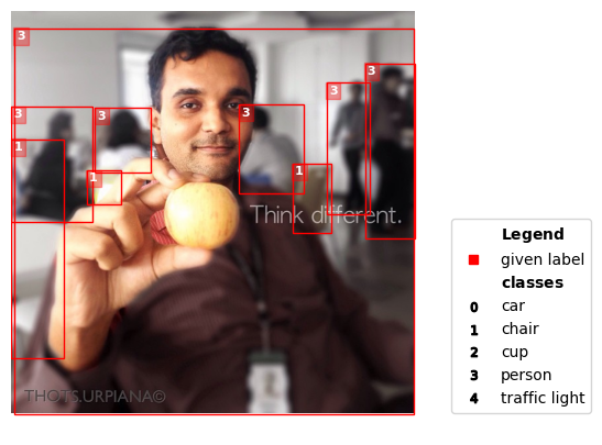
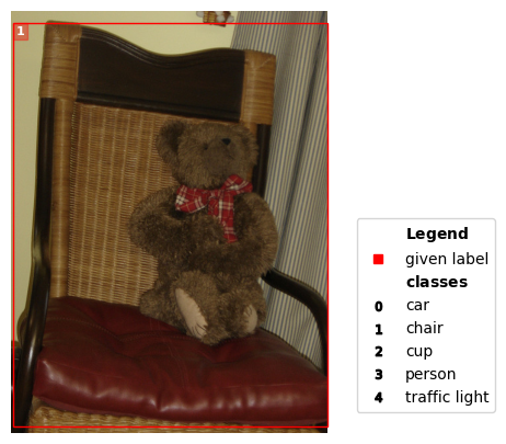
./example_images/000000395701.jpg | idx 16 | label quality score: 9.033548411774308e-05 | is issue: True
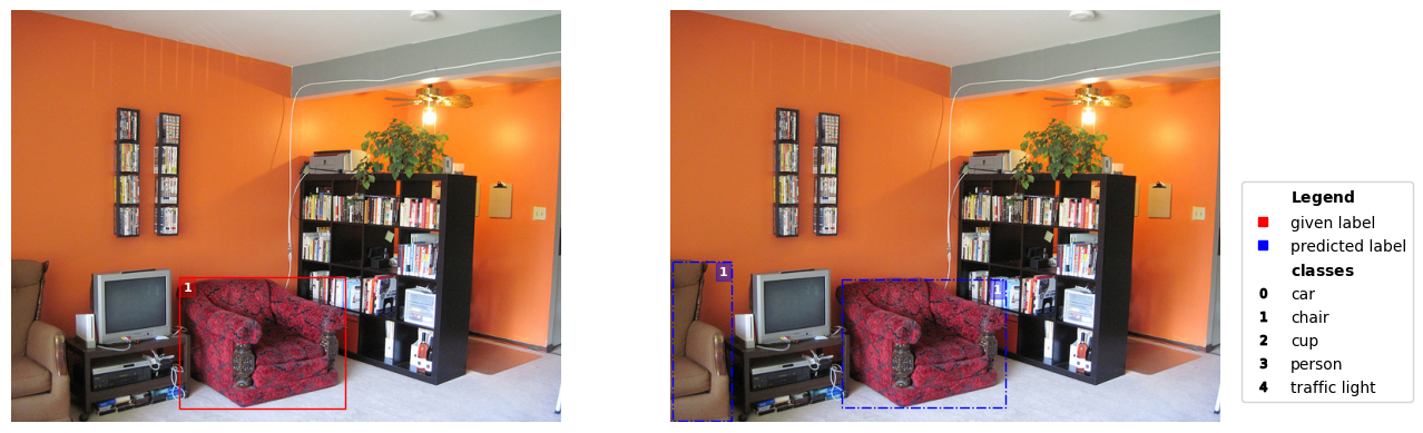
Notice the armchair to the left of the TV is missing an annotation.
[13]:
issue_to_visualize = issue_idx[9]
label = labels[issue_to_visualize]
prediction = predictions[issue_to_visualize]
score = scores[issue_to_visualize]

image_path = IMAGE_PATH + label['seg_map']
print(image_path, '| idx', issue_to_visualize , '| label quality score:', score, '| is issue: True')
if os.path.exists(image_path):
    visualize(image_path, label=label, prediction=prediction, class_names=class_names, overlay=False)
else:
    print(f"Image file not found: {image_path}")
    print("Skipping visualization - this is expected during documentation build.")
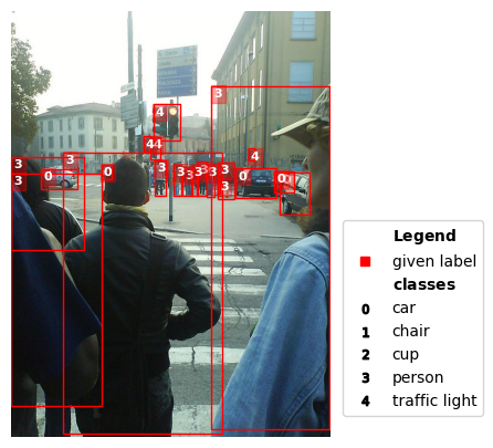
./example_images/000000154004.jpg | idx 62 | label quality score: 0.38300759625496356 | is issue: True
Similarly, the woman in a red jacket in the foreground is missing an annotation.
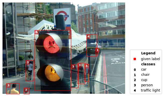
[14]:
issue_to_visualize = issue_idx[2]
label = labels[issue_to_visualize]
prediction = predictions[issue_to_visualize]
score = scores[issue_to_visualize]

image_path = IMAGE_PATH + label['seg_map']
print(image_path, '| idx', issue_to_visualize , '| label quality score:', score, '| is issue: True')
if os.path.exists(image_path):
    visualize(image_path, label=label, prediction=prediction, class_names=class_names, overlay=False)
else:
    print(f"Image file not found: {image_path}")
    print("Skipping visualization - this is expected during documentation build.")
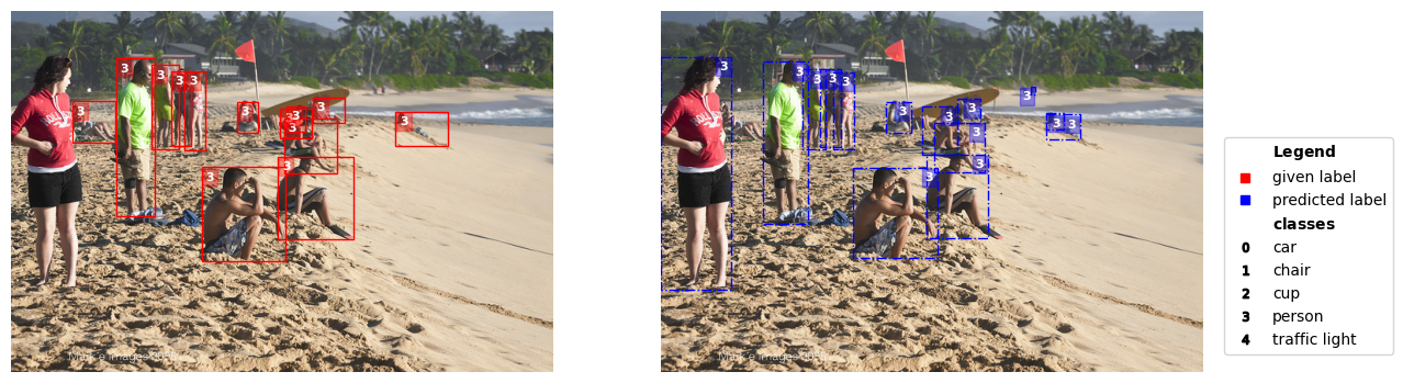
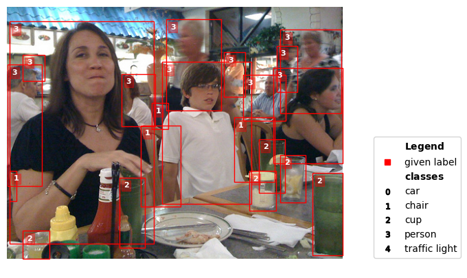
./example_images/000000448410.jpg | idx 31 | label quality score: 0.0008575101690203273 | is issue: True
The people in this image should have had individual bounding boxes around each persons (the COCO guidelines state only groups with 10+ objects of the same type can be a “crowd” bounded by a single box). Individuals in the back are missing annotations.
All of these examples received low label quality scores reflecting their low annotation quality in the original dataset.
Other uses of visualize#
The visualize() function can also depict non-issue images, labels or predictions alone, or just the image itself. Let’s explore this with a few images in our dataset.
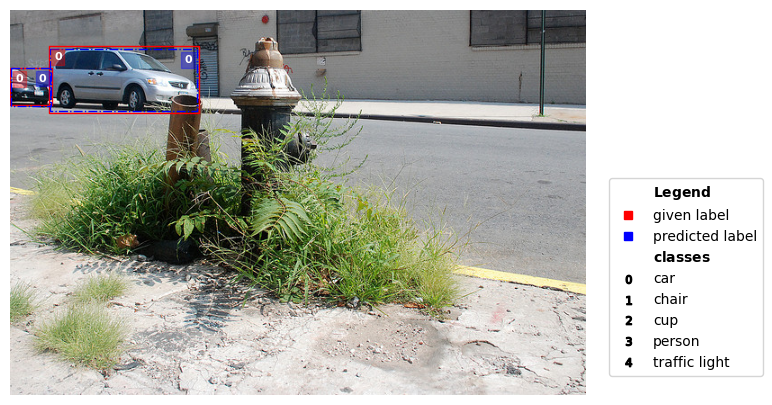
We can save a visualization to file via the save_path argument. Note the label quality score is high for this example and it is marked as a non-issue. The given and predicted labels closely resemble each other contributing to the high score.
[15]:
image_to_visualize = 0
image_path = IMAGE_PATH + labels[image_to_visualize]['seg_map']
print(image_path, '| idx', image_to_visualize , '| label quality score:', scores[image_to_visualize], '| is issue:', image_to_visualize in issue_idx)
if os.path.exists(image_path):
    visualize(image_path, label=labels[image_to_visualize], prediction=predictions[image_to_visualize], class_names=class_names, save_path='./example_image.png')
else:
    print(f"Image file not found: {image_path}")
    print("Skipping visualization - this is expected during documentation build.")
./example_images/000000499768.jpg | idx 0 | label quality score: 0.9748962231208227 | is issue: False
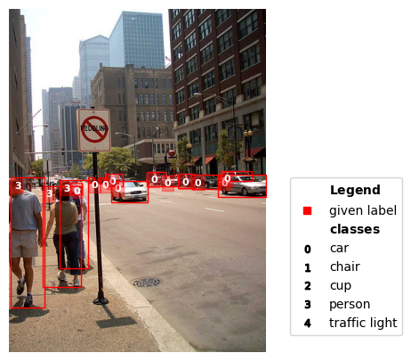
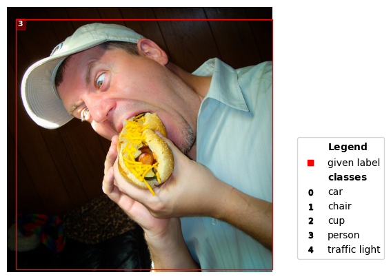
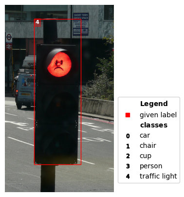
For the next example, notice how we are only passing in the given labels to visualize. We can limit visualization to either labels, predictions, or neither.
[16]:
image_to_visualize = 3
image_path = IMAGE_PATH + labels[image_to_visualize]['seg_map']
print(image_path, '| idx', image_to_visualize , '| label quality score:', scores[image_to_visualize], '| is issue:', image_to_visualize in issue_idx)
if os.path.exists(image_path):
    visualize(image_path, label=labels[image_to_visualize], class_names=class_names)
else:
    print(f"Image file not found: {image_path}")
    print("Skipping visualization - this is expected during documentation build.")
./example_images/000000521141.jpg | idx 3 | label quality score: 0.8889923658893665 | is issue: False
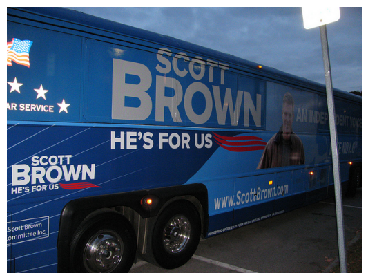
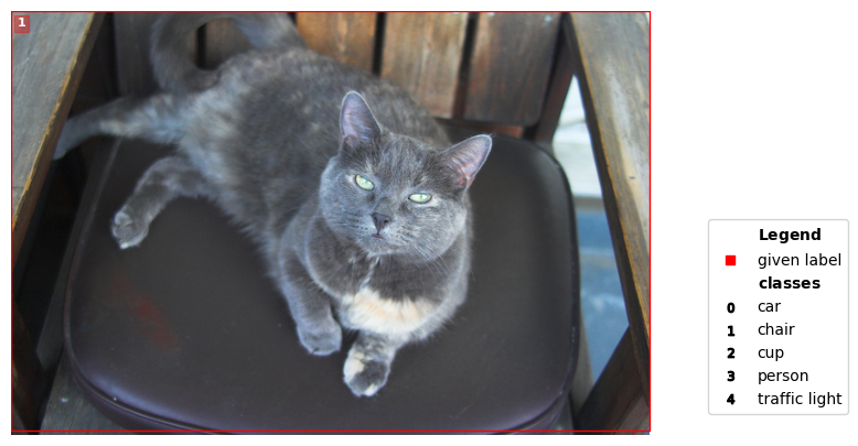
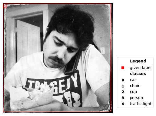
For completeness, let’s just look at an image alone.
[17]:
image_to_visualize = 2
image_path = IMAGE_PATH + labels[image_to_visualize]['seg_map']
print(image_path, '| idx', image_to_visualize , '| label quality score:', scores[image_to_visualize], '| is issue:', image_to_visualize in issue_idx)
if os.path.exists(image_path):
    visualize(image_path)
else:
    print(f"Image file not found: {image_path}")
    print("Skipping visualization - this is expected during documentation build.")
./example_images/000000143931.jpg | idx 2 | label quality score: 0.9876495074395956 | is issue: False
Exploratory data analysis#
This bonus section considers techniques to uncover annotation irregularities through exploratory data analysis. Specifically, we consider anomalies in object sizes, detect images with unusual object counts, and examine the distribution of class labels.
Let’s first consider the number of objects per image, and inspect the images with the largest values (which might reveal something off in our dataset):
[18]:
import numpy as np
from cleanlab.internal.object_detection_utils import calculate_bounding_box_areas
from cleanlab.object_detection.summary import (
    bounding_box_size_distribution,
    class_label_distribution,
    object_counts_per_image,
)
[19]:
num_imgs_to_show = 3
lab_object_counts,pred_object_counts = object_counts_per_image(labels,predictions)
for image_to_visualize in np.argsort(lab_object_counts)[::-1][0:num_imgs_to_show]:
    image_path = IMAGE_PATH + labels[image_to_visualize]['seg_map']
    print(image_path, '| idx', image_to_visualize)
    if os.path.exists(image_path):
        visualize(image_path, label=labels[image_to_visualize], class_names=class_names)
    else:
        print(f"Image file not found: {image_path}")
        print("Skipping visualization - this is expected during documentation build.")
./example_images/000000430073.jpg | idx 100
./example_images/000000183709.jpg | idx 102
./example_images/000000189475.jpg | idx 101
Next let’s study the distribution of class labels in the overall annotations, comparing the distribution in the given annotations vs. in the model predictions. This can sometimes reveal that something’s off in our dataset or model.
[20]:
label_norm,pred_norm = class_label_distribution(labels,predictions)
print("Frequency of each class amongst annotated | predicted bounding boxes in the dataset:\n")
for i in label_norm:
    print(f"{class_names[str(i)]} : {label_norm[i]} | {pred_norm[i]}")
Frequency of each class amongst annotated | predicted bounding boxes in the dataset:

car : 0.08 | 0.06
person : 0.68 | 0.7
cup : 0.11 | 0.11
chair : 0.1 | 0.09
traffic light : 0.03 | 0.04
Finally, let’s consider the distribution of bounding box sizes (aka object sizes) in the given annotations for each class label. The idea is to review any anomalies in bounding box areas for a given class (which might reveal problematic annotations or abnormal instances of this object class). The following code determines such anomalies by assessing each bounding box’s area vs. the mean and standard deviation of areas for bounding boxes with the same class label.
[21]:
lab_area,pred_area = bounding_box_size_distribution(labels,predictions)
lab_area_mean = {i: np.mean(lab_area[i]) for i in lab_area.keys()}
lab_area_std = {i: np.std(lab_area[i]) for i in lab_area.keys()}

max_deviation_values = []
max_deviation_classes = []

for label in labels:
    bounding_boxes, label_names = _separate_label(label)
    areas = calculate_bounding_box_areas(bounding_boxes)
    deviation_values = []
    deviation_classes = []

    for class_name, mean_area, std_area in zip(lab_area_mean.keys(), lab_area_mean.values(), lab_area_std.values()):
        class_areas = areas[label_names == class_name]
        deviations_away = (class_areas - mean_area) / std_area
        deviation_values.extend(list(deviations_away))
        deviation_classes.extend([class_name] * len(class_areas))

    if deviation_values==[]:
        max_deviation_values.append(0.0)
        max_deviation_classes.append(-1)
    else:
        max_deviation_index = np.argmax(np.abs(deviation_values))
        max_deviation_values.append(deviation_values[max_deviation_index])
        max_deviation_classes.append(deviation_classes[max_deviation_index])

max_deviation_classes, max_deviation_values = np.array(max_deviation_classes), np.array(max_deviation_values)
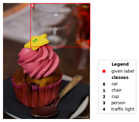
In our dataset here, this analysis reveals certain abnormally large bounding boxes that take up most of the image.
[22]:
num_imgs_to_show_per_class = 3

for c in class_names.keys():
    class_num = int(c)
    sorted_indices = np.argsort(max_deviation_values)[::-1]
    count = 0

    for i in sorted_indices:
        if max_deviation_values[i] == 0 or max_deviation_classes[i] != class_num:
            continue
        image_path = IMAGE_PATH + labels[i]['seg_map']
        print(image_path, '| idx', i, '| class', class_names[c])
        if os.path.exists(image_path):
            visualize(image_path, label=labels[i], class_names=class_names)
        else:
            print(f"Image file not found: {image_path}")
            print("Skipping visualization - this is expected during documentation build.")

        count += 1
        if count == num_imgs_to_show_per_class:
            break  # Break the loop after visualizing the top 3 instances for the current class
./example_images/000000407083.jpg | idx 115 | class car

./example_images/000000260925.jpg | idx 116 | class car

./example_images/000000065485.jpg | idx 117 | class car
./example_images/000000057232.jpg | idx 109 | class chair
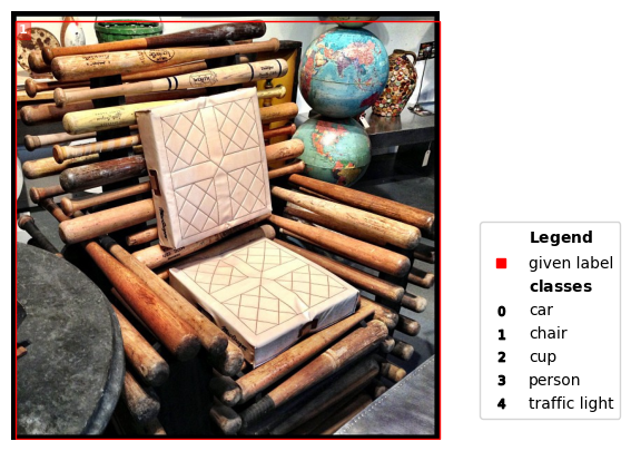
./example_images/000000044068.jpg | idx 110 | class chair
./example_images/000000353970.jpg | idx 111 | class chair
./example_images/000000463283.jpg | idx 106 | class cup
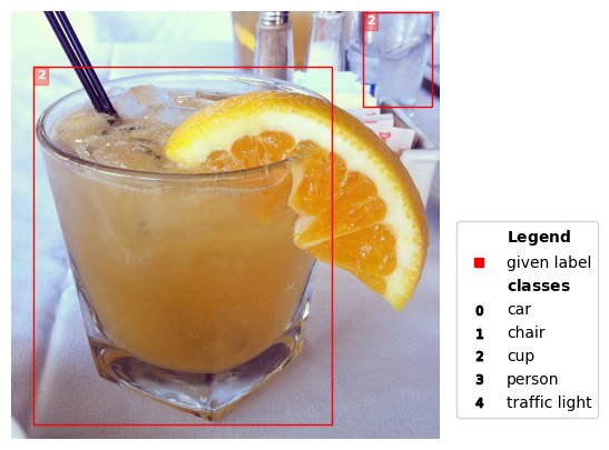
./example_images/000000331569.jpg | idx 107 | class cup
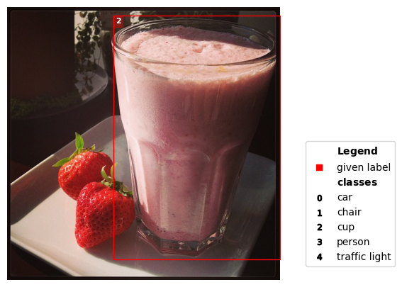
./example_images/000000450100.jpg | idx 108 | class cup
./example_images/000000422886.jpg | idx 103 | class person
./example_images/000000341828.jpg | idx 104 | class person
./example_images/000000461009.jpg | idx 105 | class person

./example_images/000000069138.jpg | idx 112 | class traffic light
./example_images/000000531134.jpg | idx 113 | class traffic light
./example_images/000000361103.jpg | idx 114 | class traffic light