Detect Outliers with Cleanlab and PyTorch Image Models (timm)

This quickstart tutorial shows how to detect outliers (out-of-distribution examples) in image data, using the cifar10 dataset as an example. You can easily replace the image dataset + neural network used here with any other Pytorch dataset + neural network (e.g. to instead detect outliers in text data with minimal code changes).

Overview of what we’ll do in this tutorial:

Detect outliers using feature_embeddings

• Pre-process cifar10 into Pytorch datasets where train_data only contains images of animals and test_data contains images from all classes.

• Use a pretrained neural network model from timm to extract feature embeddings of each image.

• Use cleanlab to find naturally occurring outlier examples in the train_data (i.e. atypical images).

• Find outlier examples in the test_data that do not stem from training data distribution (including out-of-distribution non-animal images).

• Explore threshold selection for determining which images are outliers vs not.

Detect outliers using pred_probs from a trained classifier

• Adapt our timm network into a classifier by training an additional output layer using the (in-distribution) training data.

• Use cleanlab to find out-of-distribution examples in the dataset based on the probabilistic predictions of this classifier, as an alternative to relying on feature embeddings.

Quickstart

Already have numeric feature embeddings for your data? Just run the code below to score how out-of-distribution each example is.

from cleanlab.outlier import OutOfDistribution

ood = OutOfDistribution()

# To get outlier scores for train_data using feature matrix train_feature_embeddings
ood_train_feature_scores = ood.fit_score(features=train_feature_embeddings)

# To get outlier scores for additional test_data using feature matrix test_feature_embeddings
ood_test_feature_scores = ood.score(features=test_feature_embeddings)

Already have pred_probs and labels for your classification dataset? Just run the code below to to score how out-of-distribution each example is.

from cleanlab.outlier import OutOfDistribution

ood = OutOfDistribution()

# To get outlier scores for train_data using predicted class probabilities (from a trained classifier) and given class labels
ood_train_predictions_scores = ood.fit_score(pred_probs=train_pred_probs, labels=labels)

# To get outlier scores for additional test_data using predicted class probabilities
ood_test_predictions_scores = ood.score(pred_probs=test_pred_probs)

1. Install the required dependencies

You can use pip to install all packages required for this tutorial as follows:

!pip install matplotlib sklearn torch torchvision timm
!pip install cleanlab
...
# Make sure to install the version corresponding to this tutorial
# E.g. if viewing master branch documentation:
#     !pip install git+https://github.com/cleanlab/cleanlab.git

Let’s first import the required packages

import numpy as np
import matplotlib.pyplot as plt
from pylab import rcParams
import torch
import torchvision
import timm
from sklearn import preprocessing
from sklearn.linear_model import LogisticRegression
from sklearn.ensemble import BaggingClassifier
from sklearn.model_selection import train_test_split

from cleanlab.outlier import OutOfDistribution
from cleanlab.rank import find_top_issues

2. Pre-process the Cifar10 dataset

Each image in the original cifar10 dataset belongs to 1 of 10 classes: [airplane, automobile, bird, cat, deer, dog, frog, horse, ship, truck]. After loading the data and processing the images, we manually remove some classes from the training dataset thereby making images from these classes outliers in the test dataset. Here we to remove all classes that are not an animal, such that test images from the following classes would be out-of-distribution: [airplane, automobile, ship, truck].

# Load cifar10 images into tensors for training (rescales pixel values to [0,1] interval):
transform_normalize = torchvision.transforms.Compose(
    [torchvision.transforms.ToTensor(),])

train_data = torchvision.datasets.CIFAR10(root='./data', train=True,
                                        download=True, transform=transform_normalize)
test_data = torchvision.datasets.CIFAR10(root='./data', train=False,
                                       download=True, transform=transform_normalize)

# Define in (animal) vs out (non-animal) of distribution labels
animal_classes = [2,3,4,5,6,7]  # labels correspond to animal images
non_animal_classes = [0,1,8,9]  # labels that correspond to non-animal images

# Remove non-animal images from the training dataset
animal_idxs = np.where(np.isin(train_data.targets, animal_classes))[0]

# Only work with small subset of each dataset to speedup tutorial
train_idxs = np.random.choice(animal_idxs, len(animal_idxs) // 6, replace=False)
test_idxs = np.random.choice(range(len(test_data)), len(test_data) // 10, replace=False)

train_data  = torch.utils.data.Subset(train_data, train_idxs)  # select subset of animal images for train_data
test_data  = torch.utils.data.Subset(test_data, test_idxs)  # select subset of all images for test_data
print('train_data length: %s' % (len(train_data)))
print('test_data length: %s' % (len(test_data)))

Downloading https://www.cs.toronto.edu/~kriz/cifar-10-python.tar.gz to ./data/cifar-10-python.tar.gz

Extracting ./data/cifar-10-python.tar.gz to ./data
Files already downloaded and verified
train_data length: 5000
test_data length: 1000

Visualize some of the training and test examples

See the implementation of plot_images and visualize_outliers (click to expand)

# Note: This pulldown content is for docs.cleanlab.ai, if running on local Jupyter or Colab, please ignore it.

txt_classes = {0: 'airplane',
              1: 'automobile',
              2: 'bird',
              3: 'cat',
              4: 'deer',
              5: 'dog',
              6: 'frog',
              7: 'horse',
              8:'ship',
              9:'truck'}

def imshow(img):
    npimg = img.numpy()
    return np.transpose(npimg, (1, 2, 0))

def plot_images(dataset, show_labels=False):
    plt.rcParams["figure.figsize"] = (9,7)
    for i in range(15):
        X,y = dataset[i]
        ax = plt.subplot(3,5,i+1)
        if show_labels:
            ax.set_title(txt_classes[int(y)])
        ax.imshow(imshow(X))
        ax.axis('off')
    plt.show()

def visualize_outliers(idxs, data):
    data_subset = torch.utils.data.Subset(data, idxs)
    plot_images(data_subset)

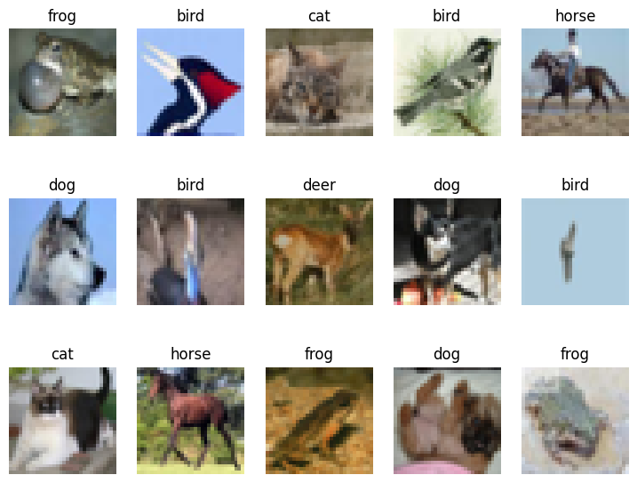
Observe how there are only animals left in our train_data:

plot_images(train_data, show_labels=True)

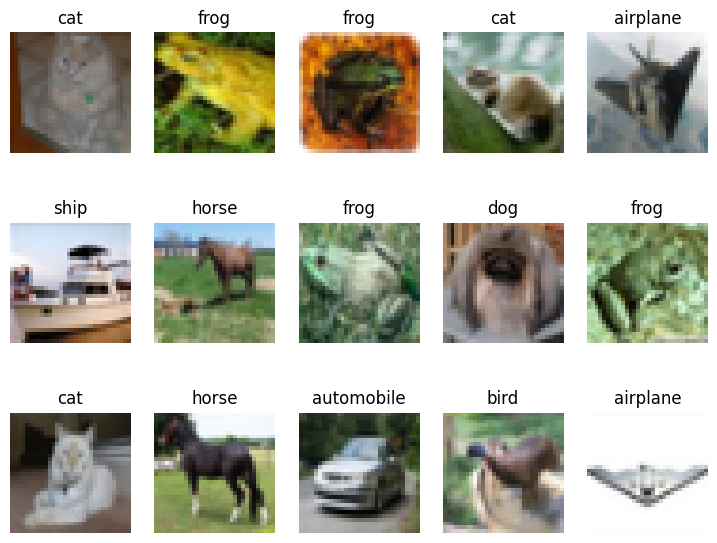
If we consider train_data to be representative of the typical data distribution, then non-animal images in test_data become outliers:

plot_images(test_data, show_labels=True)

3. Use cleanlab and feature embeddings to find outliers in the data

We can pass images through a neural network to generate vector embeddings via its hidden layer representation. Here we use a resnet50 network from timm, which has been pretrained on a large corpus of other images. Note that cleanlab’s outlier detection can be applied to numeric feature embeddings generated from any model (or to the raw data features if they are already numeric vectors). Outlier detection works best with feature vectors whose values along each dimension are of a similar scale.

# Generates 2048-dimensional feature embeddings from images
def embed_images(model, dataloader):
    feature_embeddings = []
    for data in dataloader:
        images, labels = data
        with torch.no_grad():
            embeddings = model(images)
            feature_embeddings.extend(embeddings.numpy())
    feature_embeddings = np.array(feature_embeddings)
    return feature_embeddings  # each row corresponds to embedding of a different image

# Load pretrained neural network
model = timm.create_model('resnet50', pretrained=True, num_classes=0)  # this is a pytorch network
model.eval()  # eval mode disables training-time operators (like batch normalization)

# Use dataloaders to stream images through the network
batch_size = 50
trainloader = torch.utils.data.DataLoader(train_data, batch_size=batch_size, shuffle=False)
testloader = torch.utils.data.DataLoader(test_data, batch_size=batch_size, shuffle=False)

# Generate feature embeddings
train_feature_embeddings = embed_images(model, trainloader)
print(f'Train embeddings pooled shape: {train_feature_embeddings.shape}')
test_feature_embeddings = embed_images(model, testloader)
print(f'Test embeddings pooled shape: {test_feature_embeddings.shape}')

Downloading: "https://github.com/rwightman/pytorch-image-models/releases/download/v0.1-rsb-weights/resnet50_a1_0-14fe96d1.pth" to /home/runner/.cache/torch/hub/checkpoints/resnet50_a1_0-14fe96d1.pth

Train embeddings pooled shape: (5000, 2048)
Test embeddings pooled shape: (1000, 2048)

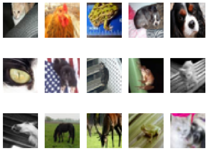
Fitting cleanlab’s OutOfDistribution class on feature_embeddings will find any naturally occurring outliers in a given dataset. These examples are atypical images that look strange or different from the majority of examples in the dataset. In our case, these correspond to odd-looking images of animals that do not resemble typical animals depicted in cifar10. This method produces a score in [0,1] for each example, where lower values correspond to more atypical examples (more likely out-of-distribution).

ood = OutOfDistribution()
train_ood_features_scores = ood.fit_score(features=train_feature_embeddings)

top_train_ood_features_idxs = find_top_issues(quality_scores=train_ood_features_scores, top=15)
visualize_outliers(top_train_ood_features_idxs, train_data)

Fitting OOD estimator based on provided features ...

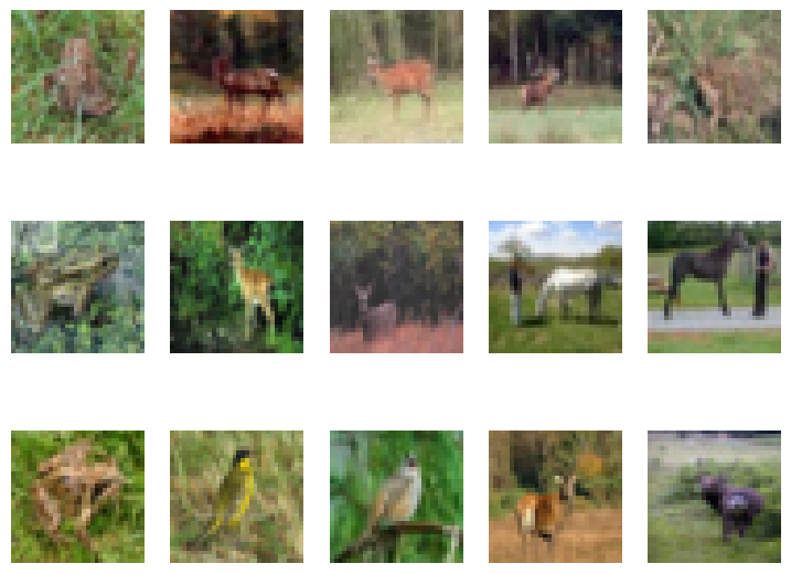
For fun, let’s see what cleanlab considers the least likely outliers in the dataset! We can do this by calling find_top_issues on the negated outlier scores. These examples look quite homogeneous as each one is similar to many other training images.

bottom_train_ood_features_idxs = find_top_issues(quality_scores=-train_ood_features_scores, top=15)
visualize_outliers(bottom_train_ood_features_idxs, train_data)

Now suppose we want to find outlier images in some never before seen test data, in particular images unlikely to stem from the same distribution as the training data. We can use our already fitted OutOfDistribution estimator to score how typical each new test example would be under the training data distribution and visualize the most severe outliers in this additional data.

test_ood_features_scores = ood.score(features=test_feature_embeddings)

top_ood_features_idxs = find_top_issues(test_ood_features_scores, top=15)
visualize_outliers(top_ood_features_idxs, test_data)

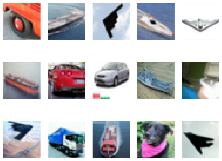
Many outliers identified in test_data depict (non-animal) classes not present in the training set. These non-animal images have very different feature embeddings than the animal-only images in the training data.

Given outlier scores, how do we determine how many of the top-ranked examples in test_data should be marked as outliers?

Inevitably this has some true positive / false positive trade-off, so let’s suppose we want to ensure around at most 5% false positives. We can use the 5th percentile of the distribution of train_ood_features_scores (assuming the training data are in-distribution examples without outliers) as a hard score threshold below which to consider a test example an outlier.

Let’s plot the 5th percentile of the training outlier score distribution (shown as red line).

fifth_percentile = np.percentile(train_ood_features_scores, 5)  # 5th percentile of the train_data distribution

# Plot outlier_score distributions and the 5th percentile cutoff
fig, axes = plt.subplots(nrows=1, ncols=2, figsize=(12, 5))
plt_range = [min(train_ood_features_scores.min(),test_ood_features_scores.min()), \
             max(train_ood_features_scores.max(),test_ood_features_scores.max())]
axes[0].hist(train_ood_features_scores, range=plt_range, bins=50)
axes[0].set(title='train_outlier_scores distribution', ylabel='Frequency')
axes[0].axvline(x=fifth_percentile, color='red', linewidth=2)
axes[1].hist(test_ood_features_scores, range=plt_range, bins=50)
axes[1].set(title='test_outlier_scores distribution', ylabel='Frequency')
axes[1].axvline(x=fifth_percentile, color='red', linewidth=2)

plt.show()

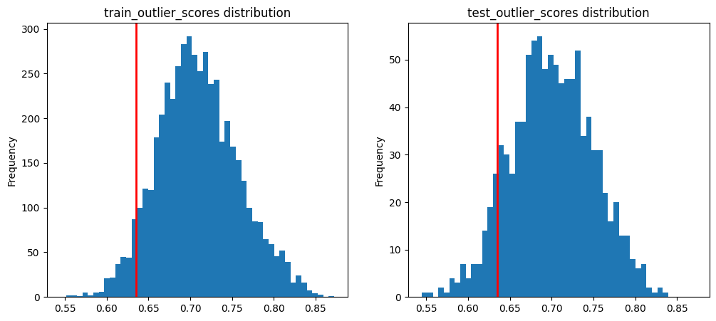
All test examples whose test_ood_features_scores fall left of the red line will be marked as an outlier.

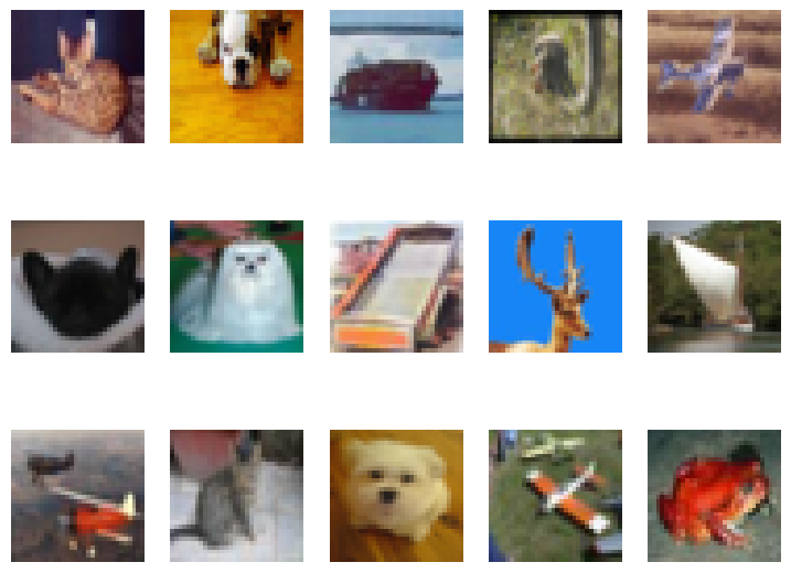
Let’s plot the least-certain outliers of our test_data (i.e. 15 images with outlier scores right along the threshold). These are the images immediately to the left of that cutoff threshold (red line). The majority of them are still truly out-of-distribution non-animal images, but there are a few atypical-looking animals that are now erroneously identified as outliers as well.

sorted_idxs = test_ood_features_scores.argsort()
ood_features_scores = test_ood_features_scores[sorted_idxs]
ood_features_indices = sorted_idxs[ood_features_scores < fifth_percentile]  # Images in test data flagged as outliers

visualize_outliers(ood_features_indices[::-1], test_data)

Outlier scores are defined relative to the average distance (computed over feature values) between each example and its K nearest neighbors in the training data. Such scores have been found to be particularly effective for out-of-distribution detection, see this paper for more details:

Back to the Basics: Revisiting Out-of-Distribution Detection Baselines

Internally, cleanlab uses the sklearn.neighbors.NearestNeighbor class (with cosine distance) to find the K nearest neighbors, but you can easily use another KNN estimator with cleanlab’s OutOfDistribution class.

4. Use cleanlab and pred_probs to find outliers in the data

We sometimes wish to find outliers in classification datasets for which we do not have meaningful numeric feature representations. In this case, cleanlab can detect unusual examples in the data solely using predicted probabilities from a trained classifier.

To get pred_probs here, a Logistic Regression classifier is fit on the already generated train_feature_embeddings (from our pretrained timm network) and the given label for each training image. We use a simple classifier here to quickly generate pred_probs, but in practice fine-tuning the entire neural network for classification will be more effective (our approach here is equivalent to only training an extra output layer appended on top of the pretrained network).

# Preprocess data
train_labels = np.array(train_data.dataset.targets)[train_data.indices]
train_labels = np.unique(train_labels, return_inverse=True)[1]  # MAKE SURE to zero index training labels for sklearn
test_labels = np.array(test_data.dataset.targets)[test_data.indices]

scaler = preprocessing.StandardScaler().fit(train_feature_embeddings)
train_feature_embeddings_scaled = scaler.transform(train_feature_embeddings)
test_feature_embeddings_scaled = scaler.transform(test_feature_embeddings)

# Our classifier employs bagging to better account for epistemic uncertainty
model = BaggingClassifier(LogisticRegression(max_iter=500), random_state=1, n_jobs=-1)
model.fit(train_feature_embeddings_scaled, train_labels)

train_pred_probs = model.predict_proba(train_feature_embeddings_scaled)
train_pred_labels = train_pred_probs.argmax(1)
accuracy = np.mean(train_pred_labels == train_labels)
print(f"Model accuracy on held-out train_data {accuracy}")

Model accuracy on held-out train_data 0.9702

We can use these pred_probs to again compute out-of-distribution scores for each image in our dataset using cleanlab’s OutOfDistribution class.

ood = OutOfDistribution()
train_ood_predictions_scores = ood.fit_score(pred_probs=train_pred_probs, labels=train_labels)

Fitting OOD estimator based on provided pred_probs ...

We can repeat this for additional test data, to identify test images that do not stem from the training data distribution.

test_pred_probs = model.predict_proba(test_feature_embeddings_scaled)

test_ood_predictions_scores = ood.score(pred_probs=test_pred_probs)

Detecting outliers based on feature embeddings can be done for arbitrary unlabeled datasets, but requires a meaningful numerical representation of the data. Detecting outliers based on predicted probabilities applies mainly for labeled classification datasets, but can be done with any effective classifier. The effectiveness of the latter approach depends on: how much auxiliary information captured in the feature values is lost in the predicted probabilities (determined by the particular set of labels in the classification task), the accuracy of our classifier, and how properly its predictions reflect epistemic uncertainty. Read more about it here.